Mathis Dubau · Scheme bank
Schemes
The 99 schemes I drew in Tik Z for my thesis, to download as PDF or SVG. Reuse them freely, citing the thesis.
Click a scheme to open it full size; under each one, PDF and SVG download it. To reuse a scheme, cite the thesis
with the figure number shown under it (one click on the box selects all of it for copying):
@phdthesis{Dubau:thesis,
  author = "M. Dubau",
  title  = "{Multivariate study of polarisation states in electroweak vector boson scattering WZ events using ATLAS data at the LHC}",
  school = "Universit\'{e} Savoie Mont Blanc",
  year   = "2026",
  doi    = "10.17181/cw32k-7w243",
  url    = "https://repository.cern/records/cw32k-7w243",
  type   = "PhD thesis"
}
The Standard Model
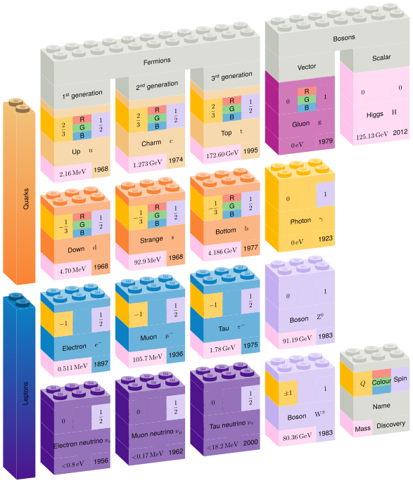
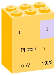
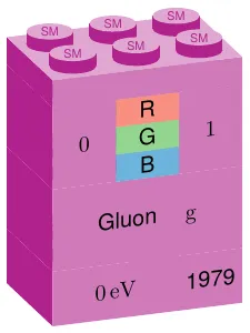
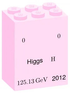
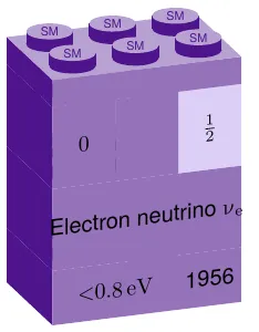
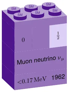
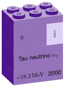
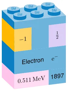
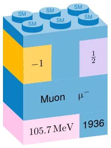
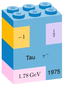
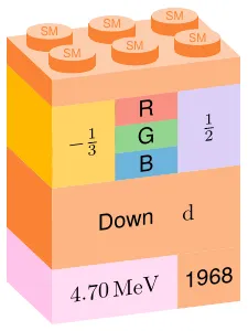
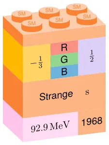
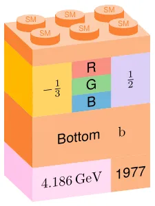
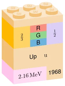
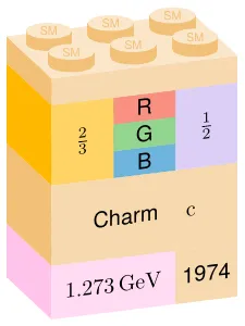
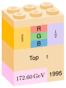
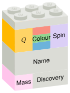
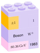
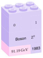
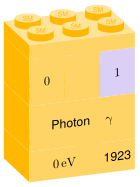
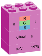
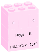
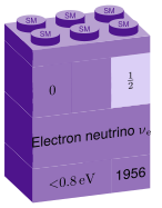
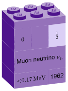
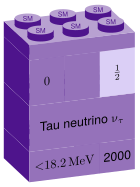
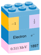
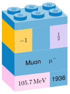
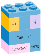
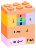
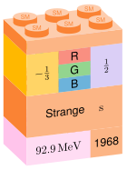
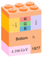
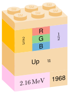
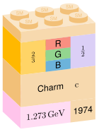
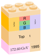
The Standard Model in Lego bricks: quarks, leptons and bosons, coloured by the interactions they take part in. Thesis Fig. 1.5 PDF · SVG
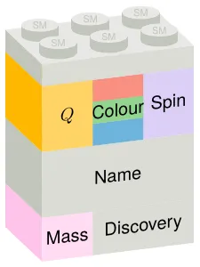
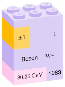
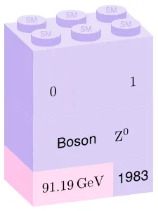
The 18 bricks, one by one
The Higgs potential: the field rolls from the unstable top to the circle of minima and breaks the symmetry. Thesis Fig. 1.2 PDF · SVG
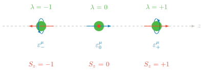
The three helicity states of a vector boson: spin − 1 -1 0 0 + 1 +1 Thesis Fig. 1.6 PDF · SVG
Feynman diagrams
Vertices and scalar scattering
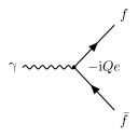
The QED vertex: a photon couples to a fermion–antifermion pair with strength − i Q e -iQe Thesis Fig. 1.1 PDF · SVG
5 more schemes
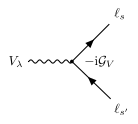
The electroweak vertex: a W or Z boson couples to a pair of fermions. Thesis Fig. C.1 PDF · SVG
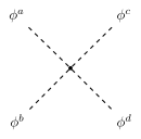
Quartic scalar interaction, the contact term of scalar scattering. Thesis Fig. A.1(a) PDF · SVG
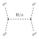
Scalar scattering through an s-channel Higgs exchange. Thesis Fig. A.1(b) PDF · SVG
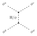
Scalar scattering through a t-channel Higgs exchange. Thesis Fig. A.1(c) PDF · SVG
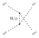
Scalar scattering through a u-channel Higgs exchange. Thesis Fig. A.1(d) PDF · SVG
Vector boson scattering
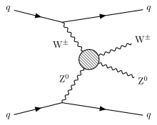
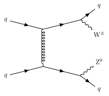
Vector boson scattering: two quarks radiate a W and a Z that scatter, leaving two forward jets. Thesis Fig. 6.4 PDF · SVG
2 more schemes
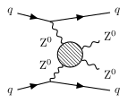
Electroweak ZZjj production through vector boson scattering. Thesis Fig. 6.17(h) PDF · SVG
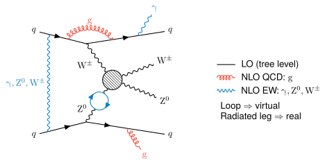
Corrections to WZjj: NLO QCD and NLO electroweak emissions, virtual and real. Thesis Fig. 6.16 PDF · SVG
Backgrounds
Show the 10 schemes
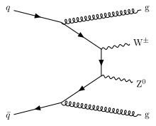
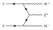
QCD-induced WZjj production, the main irreducible background. Thesis Fig. 6.5(a) PDF · SVG
Another QCD-induced WZjj diagram. Thesis Fig. 6.5(b) PDF · SVG
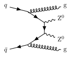
QCD-induced ZZjj production. Thesis Fig. 6.17(i) PDF · SVG
Triboson production, a background with three leptons. Thesis Fig. 6.17(e) PDF · SVG
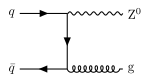
Z + jets, a background when a jet fakes the third lepton. Thesis Fig. 6.17(f) PDF · SVG
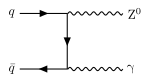
Z γ \mathrm{Z}\gamma Thesis Fig. 6.17(g) PDF · SVG
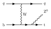
tZj production, a background with three leptons and jets. Thesis Fig. 6.17(d) PDF · SVG
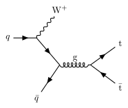
t t ‾ W \mathrm{t\bar{t}W} Thesis Fig. 6.17(b) PDF · SVG
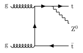
t t ‾ Z \mathrm{t\bar{t}Z} Thesis Fig. 6.17(c) PDF · SVG
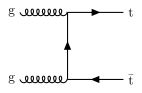
t t ‾ \mathrm{t\bar{t}} Thesis Fig. 6.17(a) PDF · SVG
Beyond the Standard Model
Show the 1 schemes
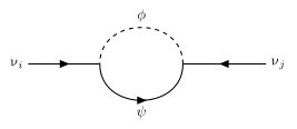
The one-loop diagram that gives neutrinos a Majorana mass in the scotogenic model. Thesis Fig. Z.1 PDF · SVG
Vector boson scattering and the WZ analysis
History
Show the 2 schemes
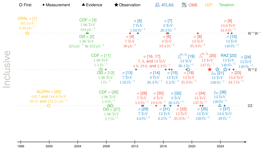
Diboson and triboson measurements at LEP, the Tevatron and the LHC over time. PDF · SVG
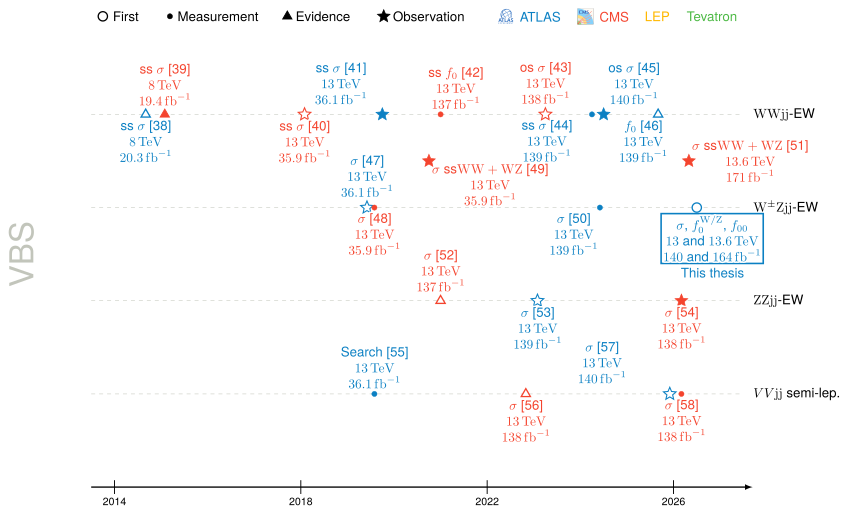
Vector boson scattering measurements over time, from searches to observations. PDF · SVG
Events and selection
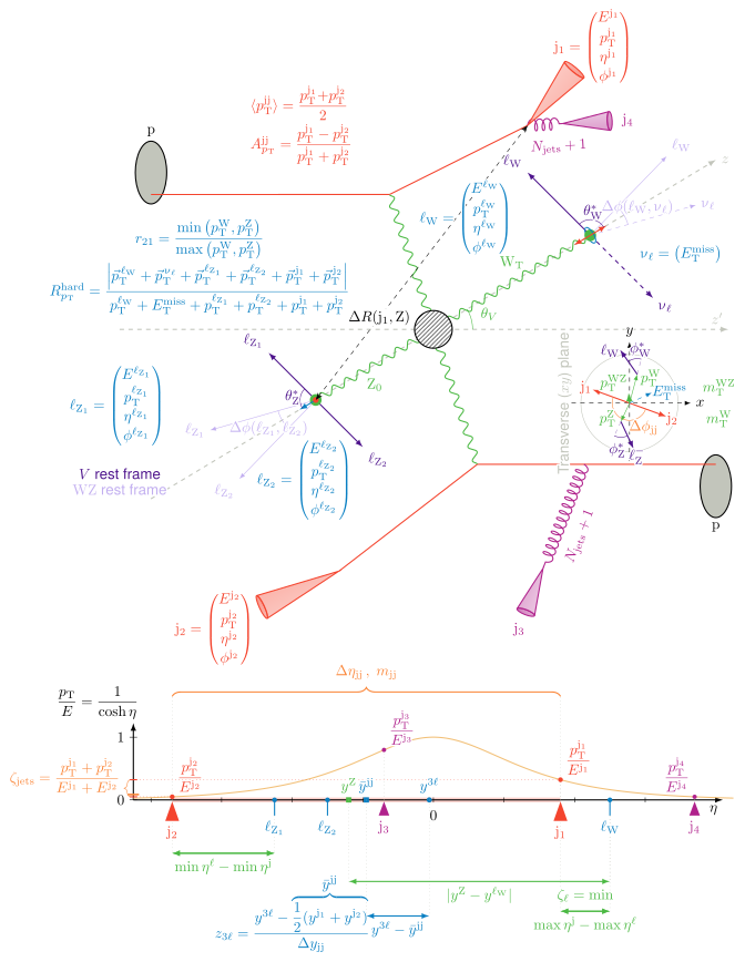
A WZjj vector boson scattering event in ATLAS. Thesis Fig. 6.15 PDF · SVG
Discriminant plane
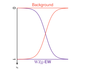
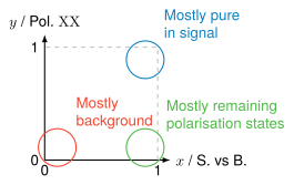
Output of the signal-versus-background network: background near 0, WZjj-EW near 1. Thesis Fig. 6.19(a) PDF · SVG
The discriminant plane: background bottom left, the targeted polarisation state top right. Thesis Fig. 6.23 PDF · SVG
3 more schemes
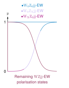
Output of a polarisation network for the targeted state and the others. Thesis Fig. 6.19(b) PDF · SVG
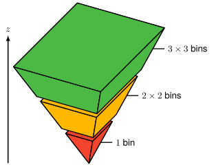
Binning the discriminant plane: 1 1 2 × 2 2\times2 3 × 3 3\times3 Thesis Fig. G.1(a) PDF · SVG
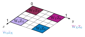
The four polarisation states of the WZ pair, longitudinal (0) or transverse (T). Thesis Fig. G.1(b) PDF · SVG
Statistics
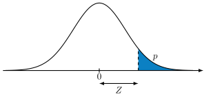
From a p p Z Z Thesis Fig. O.1 PDF · SVG
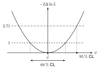
A profile-likelihood scan and the intervals read where − 2 Δ ln L -2\Delta\ln L 1 1 2.71 2.71 Thesis Fig. O.2 PDF · SVG
Machine learning
Neural networks
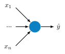
An artificial neuron: weighted inputs, a sum and an activation. Thesis Fig. 4.1 PDF · SVG
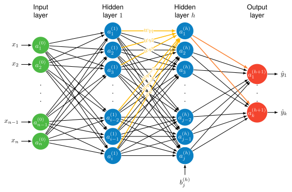
A fully connected neural network with two hidden layers. Thesis Fig. 4.2 PDF · SVG
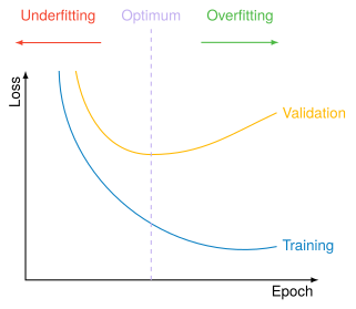
Under- and overfitting: training and validation loss against the epochs. Thesis Fig. 4.5 PDF · SVG
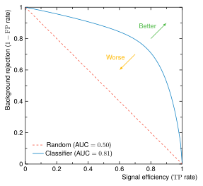
A ROC curve: background rejection against signal efficiency. Thesis Fig. 4.8 PDF · SVG
5 more schemes
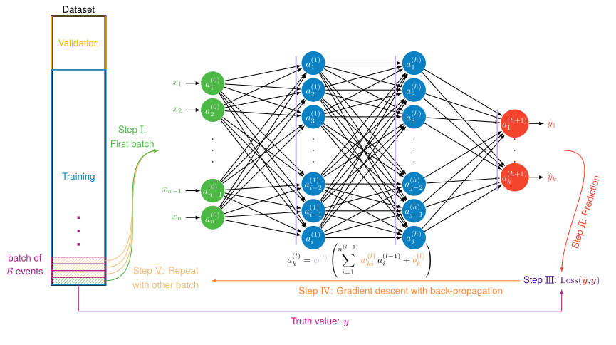
Training a network: forward pass, loss against the truth, back-propagation. PDF · SVG
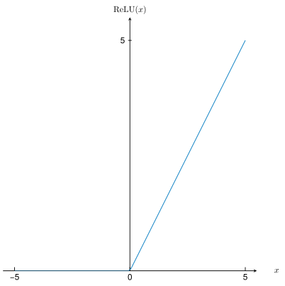
The ReLU activation. Thesis Fig. 4.4(a) PDF · SVG
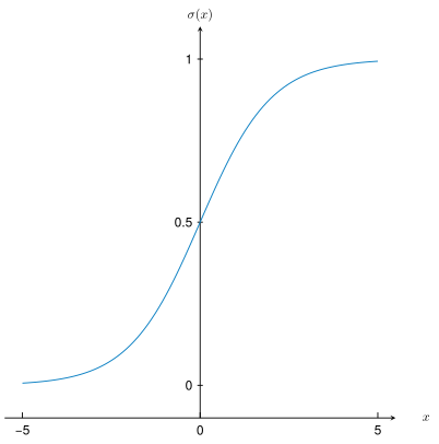
The sigmoid activation. Thesis Fig. 4.4(b) PDF · SVG
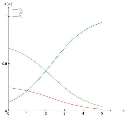
The softmax activation. Thesis Fig. 4.4(c) PDF · SVG
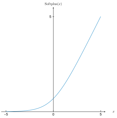
The softplus activation. Thesis Fig. 5.13 PDF · SVG
Decision trees
Show the 3 schemes
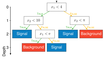
A decision tree and the cuts it makes. Thesis Fig. 4.9(a) PDF · SVG
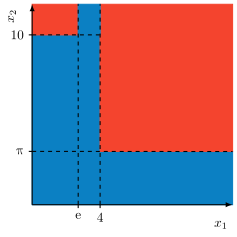
The regions a decision tree cuts the plane into. Thesis Fig. 4.9(b) PDF · SVG
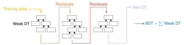
Boosting: each weak tree learns from the residuals of the previous ones. Thesis Fig. 4.10 PDF · SVG
Active learning
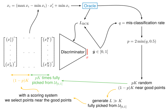
The active-learning loop: a network chooses which points the expensive oracle computes. Thesis Fig. Z.2 PDF · SVG
Simulation
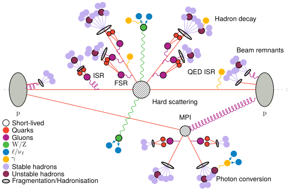
A simulated proton–proton collision: hard scattering, parton showers, underlying event and hadronisation. Thesis Fig. 4.13 PDF · SVG
CERN and the LHC
Accelerators
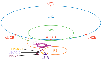
The CERN accelerator complex, from LINAC 4 to the LHC. Thesis Fig. 2.3 PDF · SVG
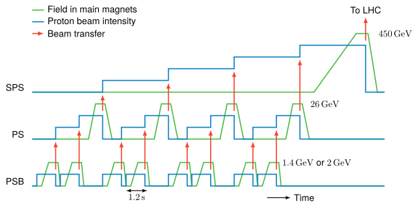
The injection chain: the magnet cycles of the PS Booster, PS and SPS that fill the LHC. Thesis Fig. 2.4(a) PDF · SVG
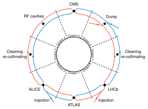
The LHC ring and its eight sectors, with the four large experiments. Thesis Fig. 2.5 PDF · SVG
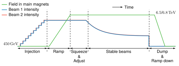
An LHC fill: injection, ramp, squeeze, stable beams and dump. Thesis Fig. 2.4(b) PDF · SVG
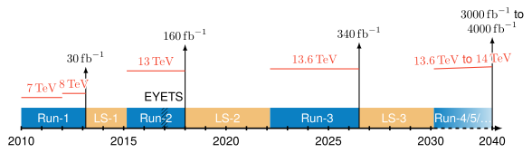
The LHC timeline, from Run 1 to the High-Luminosity LHC. Thesis Fig. 2.6 PDF · SVG
Coordinates
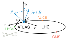
The LHC ring and the ATLAS axes. Thesis Fig. 3.2(a) PDF · SVG
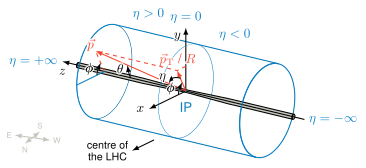
The ATLAS coordinate system and the pseudorapidity η \eta Thesis Fig. 3.2(b) PDF · SVG
The ATLAS detector
Whole detector
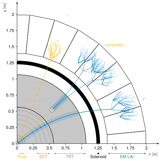
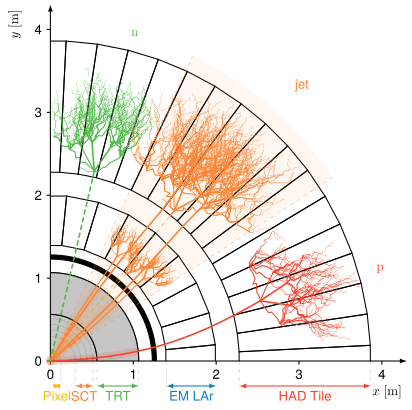
Electromagnetic showers of electrons and photons in the ATLAS calorimeter. Thesis Fig. 5.1 PDF · SVG
Hadronic showers in the ATLAS calorimeters. Thesis Fig. 6.7(a) PDF · SVG
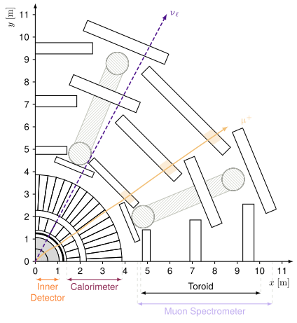
A muon crossing the whole of ATLAS. Thesis Fig. 6.7(b) PDF · SVG
Inner detector
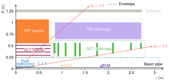
Quarter view of the ATLAS Inner Detector: pixels, strips and straw tubes. Thesis Fig. 3.3(b) PDF · SVG
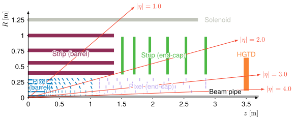
Quarter view of the ITk and HGTD, which reach | η | = 4 |\eta| = 4 Thesis Fig. 3.16(b) PDF · SVG
6 more schemes
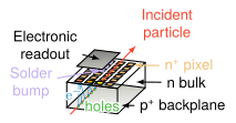
A pixel sensor and its bump-bonded readout. Thesis Fig. 3.4(a) PDF · SVG
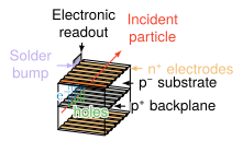
An IBL pixel sensor. Thesis Fig. 3.4(b) PDF · SVG
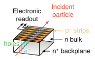
An SCT strip sensor. Thesis Fig. 3.4(c) PDF · SVG
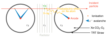
A TRT straw: ionisation and transition radiation in a gas-filled tube. Thesis Fig. 3.5 PDF · SVG
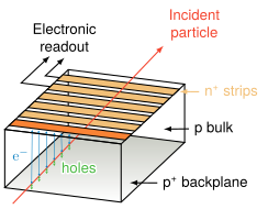
An ITk strip sensor. Thesis Fig. 3.17(a) PDF · SVG
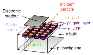
An HGTD low-gain avalanche sensor, which times each track. Thesis Fig. 3.17(b) PDF · SVG
Calorimeters
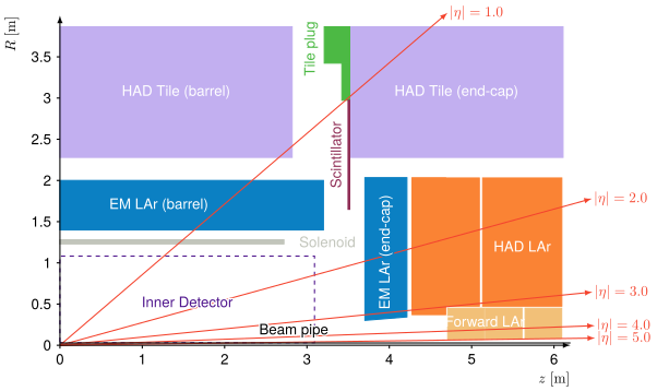
Quarter view of the ATLAS calorimeters. Thesis Fig. 3.6(b) PDF · SVG
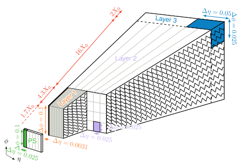
The accordion geometry of the ATLAS liquid-argon electromagnetic calorimeter. Thesis Fig. 3.7(a) PDF · SVG
4 more schemes
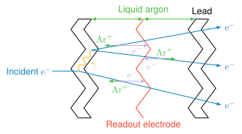
Sampling in liquid argon: lead absorbers, argon gaps and readout electrodes. Thesis Fig. 3.8(a) PDF · SVG
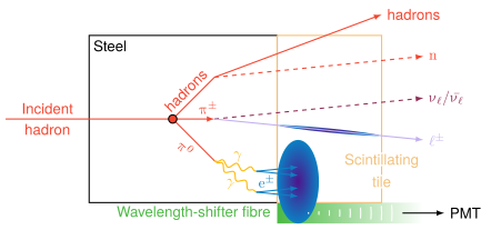
Sampling in the Tile calorimeter: steel and scintillator, read through wavelength-shifting fibres. Thesis Fig. 3.8(b) PDF · SVG
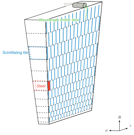
A Tile calorimeter module. Thesis Fig. 3.7(b) PDF · SVG
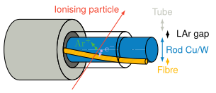
A forward calorimeter electrode: a rod in a tube, with a thin liquid-argon gap. Thesis Fig. 3.9 PDF · SVG
Muon spectrometer
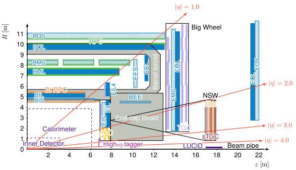
Quarter view of the ATLAS muon spectrometer. Thesis Fig. 3.10(b) PDF · SVG
5 more schemes
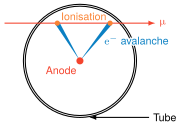
A monitored drift tube: the muon ionises the gas and the electrons drift to the anode wire. Thesis Fig. 3.11(a) PDF · SVG
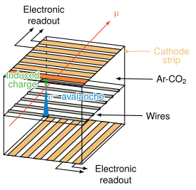
A cathode strip chamber. Thesis Fig. 3.11(b) PDF · SVG
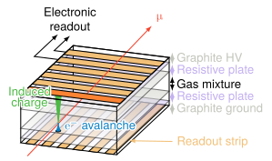
A resistive plate chamber. Thesis Fig. 3.12(a) PDF · SVG
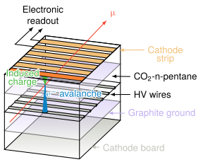
A thin gap chamber. Thesis Fig. 3.12(b) PDF · SVG
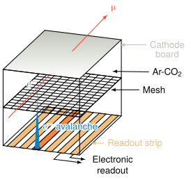
A Micromegas chamber of the New Small Wheel. Thesis Fig. 3.11(c) PDF · SVG
Trigger and luminosity
Show the 2 schemes
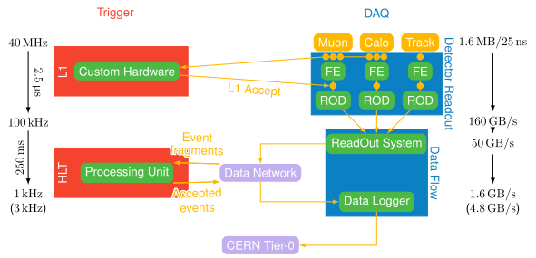
The ATLAS trigger and data acquisition chain. Thesis Fig. 3.14 PDF · SVG
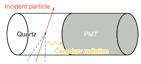
LUCID, the luminosity monitor: Cherenkov light in quartz read by photomultipliers. Thesis Fig. 3.15 PDF · SVG
Reconstruction
Tracks
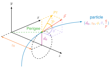
The perigee parameters of a track. Thesis Fig. 5.3 PDF · SVG
1 more scheme
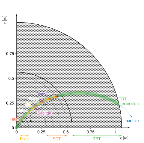
Track reconstruction in the inner detector. Thesis Fig. 5.4 PDF · SVG
Electrons and photons
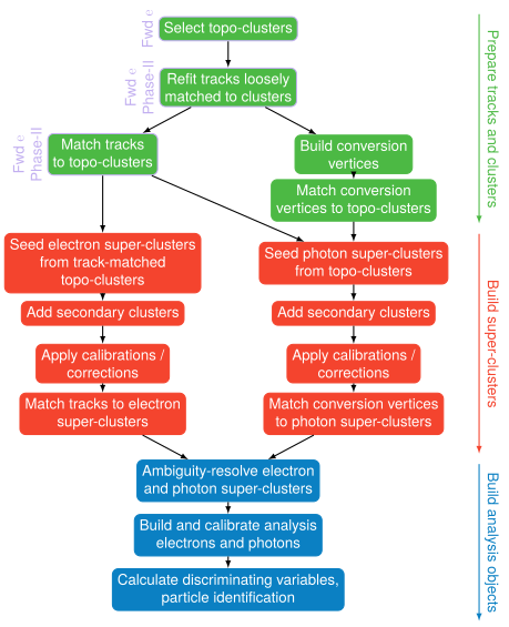
Electron and photon reconstruction in ATLAS, step by step. Thesis Fig. 5.2 PDF · SVG
8 more schemes
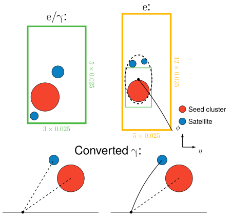
Superclusters: a seed cluster gathers its satellites, for electrons and converted photons. Thesis Fig. 5.6 PDF · SVG
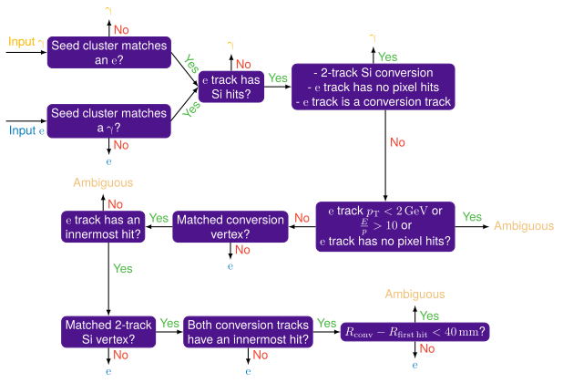
Electron or photon? How the ambiguity is resolved. Thesis Fig. 5.7 PDF · SVG
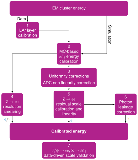
The electron and photon energy calibration chain. Thesis Fig. 5.8 PDF · SVG
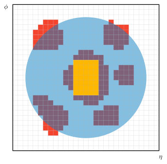
Calorimeter isolation: the energy in a cone around the electron, its core removed. Thesis Fig. 5.10 PDF · SVG
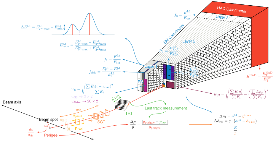
The calorimeter and track variables used to identify electrons. PDF · SVG
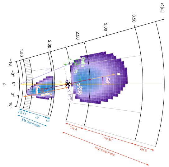
A forward electron shower and its cluster moments. Thesis Fig. 5.11 PDF · SVG
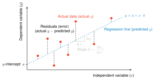
Decorrelation: a variable replaced by its residual from a linear fit in p T p_{\text{T}} Thesis Fig. 5.16 PDF · SVG
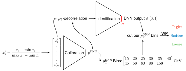
The forward-electron calibration and identification workflow. Thesis Fig. 5.18 PDF · SVG
Jets, muons, taus and missing momentum
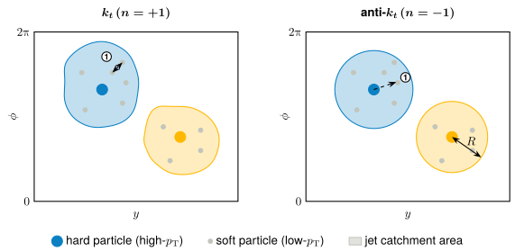
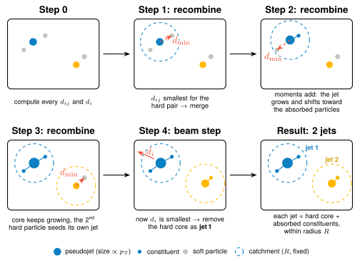
k t k_t k t k_t k t k_t Thesis Fig. 6.9(a) PDF · SVG
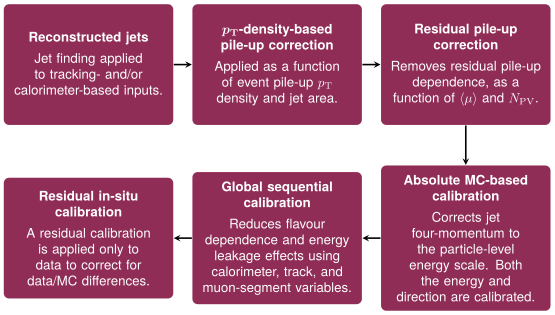
The ATLAS jet energy calibration chain. Thesis Fig. 6.10 PDF · SVG
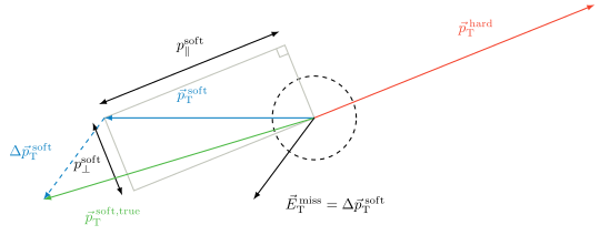
Missing transverse momentum: minus the vector sum of every reconstructed object. Thesis Fig. 6.12 PDF · SVG
6 more schemes
The k t k_t Thesis Fig. 6.9(b) PDF · SVG
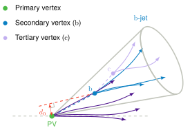
A b-jet: the b hadron flies before decaying at a secondary vertex. Thesis Fig. 6.11(a) PDF · SVG
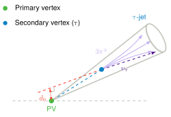
A τ \tau Thesis Fig. 6.11(b) PDF · SVG
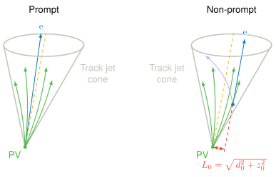
Prompt and non-prompt leptons: a lepton from a secondary vertex is displaced from the primary one. Thesis Fig. 5.5 PDF · SVG
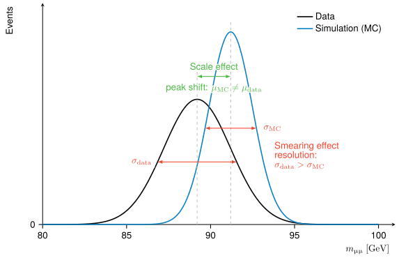
Muon momentum corrections: the simulation is matched to the data on the Z peak. Thesis Fig. 6.6 PDF · SVG
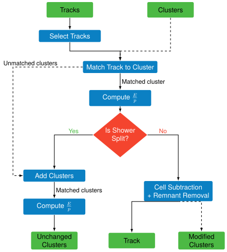
Particle flow: tracks are matched to calorimeter clusters and their expected energy is subtracted. Thesis Fig. 6.8 PDF · SVG
Drawn with the thesis, not printed in it
Show the 9 schemes
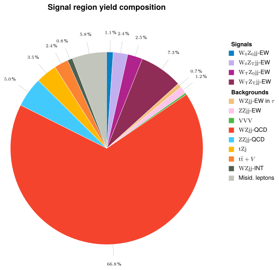
What the signal region is made of: the WZjj signal and each background. PDF · SVG
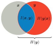
The information budget: what the inputs x x y y I ( x ; y ) I(x;y) H ( y | x ) H(y|x) PDF · SVG
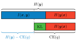
A cross-entropy gives a lower bound on the mutual information: I ( x ; y ) ≥ H ( y ) − C E ( q ) I(x;y) \geq H(y) - \mathrm{CE}(q) PDF · SVG
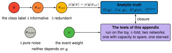
The toy model used to check the information measurements against the analytic truth. PDF · SVG
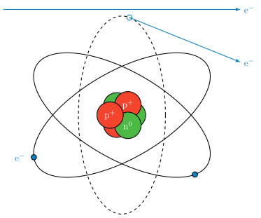
Ionisation: a charged particle passing by knocks an electron out of the atom. PDF · SVG
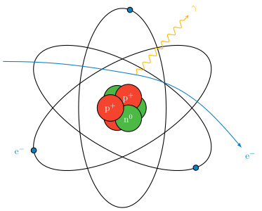
Bremsstrahlung: an electron deflected by the nucleus radiates a photon. PDF · SVG
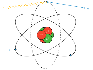
Photoelectric effect: a photon is absorbed and ejects a bound electron. PDF · SVG
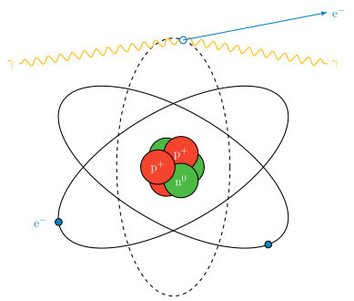
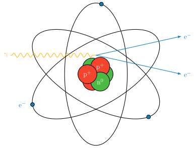
Compton scattering: a photon scatters off an atomic electron and loses energy. PDF · SVG
Pair creation: near a nucleus, a photon turns into an electron–positron pair. PDF · SVG